RP ProPulse – Numerical Simulation of Pulse Propagation
| Overview | Purpose | Model | Interface | Demos | Versions |
Example Case: Active Mode Locking
In this simple example, we consider an actively mode-locked laser. The laser resonator is described in the script as follows:
resonator: ring
* Crystal: gain(l) = g(l)
   [P_sat_av = P_sat_g, KK = 0]
* Modulator: mod(t) = t_mod(t)
* OC: T_out = T_OC
resonator end
This refers to some variable values, the definitions of which are not shown here. The gain function g(l) has a limited bandwidth of 0.2 nm, and the modulator modulates the resonator round-trip losses with 100 MHz and peak losses of 10%.
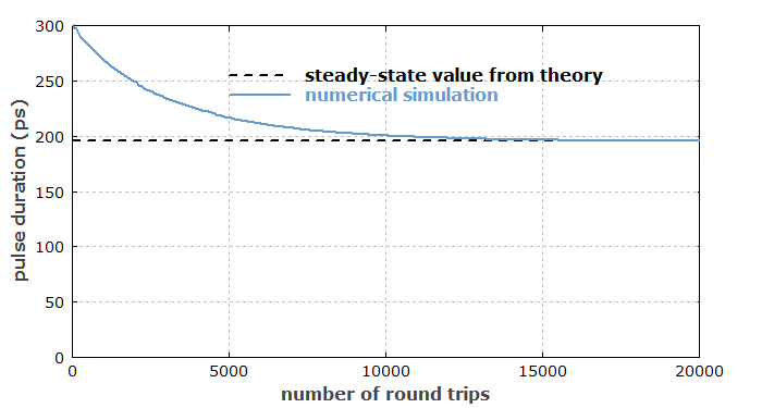
The initial pulse duration was chosen to be somewhat longer than in the steady state. It is found that the steady-state value of the pulse duration agrees with the result of Kuizenga–Siegman theory (see the diagram below).

The script code required for that diagram is pretty simple:
; ---------------------------
diagram 1:

"Evolution of Pulse Parameters"

x: 0, 20000
"number of round trips", @x
y: 0, 300
"pulse duration (ps)", @y
frame
legpos 200, 160
hx
hy

tau_th := 0.45 *
  ((0.5 * T_OC) / (0.25 * A_mod))^0.25
  / sqrt(f_mod * df_g)
 { theoretical value for steady-state
   pulse duration according to
   Kuizenga-Siegman theory }

f: tau_th / ps,
  "steady-state value from theory",
  style = dashed, width = 3

f: (getpulse(x / rt_per_step,0);
    tau()) / ps,
  "numerical simulation",
  color = blue, width = 3
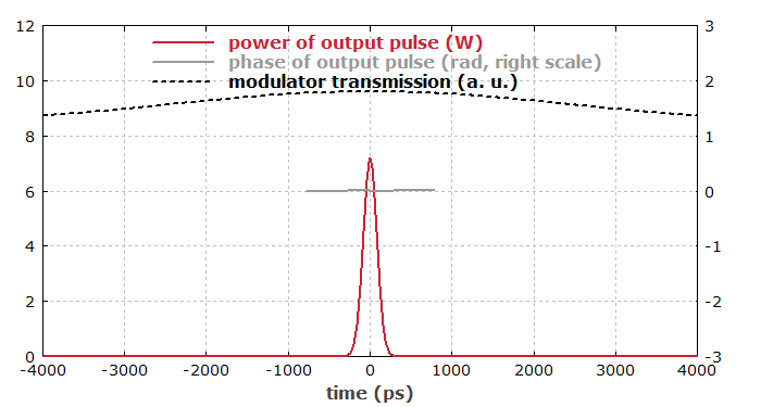
Also, we can see the temporal pulse profile after 2000 resonator round trips (which are calculated within a few seconds on an ordinary PC):

