
![]()
RP Fiber Power – Simulation and Design Software
for Fiber Optics, Amplifiers and Fiber Lasers
| Overview | Features | Speed | Model |
| Data | Interface | Demos | Versions |
Example Case: Launching Light into a Single-mode Fiber
Description of the Model
We simulate the following case:
- We have a single-mode fiber with a step-index profile.
- We focus a monochromatic Gaussian beam with a beam radius of 3 μm onto the input end. Even for perfect alignment, that beam profile does not perfectly fit the guided fiber mode. In addition, the input beam may be somewhat offset from the core position.
Some technical details of the simulation:
- For the beam propagation, we introduce an artificial loss outside the core region (increasing towards to the grid boundaries) which simulates the losses for cladding modes.
- We use the mode solver to get the profile of the fundamental mode. For comparison with the numerical results, we analytically calculate the mode overlap of the input beam, from which we obtain the expected launch efficiency.
Note that while the mode solver is limited to cases with radial symmetry of the refractive index profile, them beam propagation could be calculated for arbitrary index profiles, as long as they are weakly guiding (which is essentially the case for all all-glass fibers).
Setting up the beam propagation with a few lines of script code is simple, after some parameters have been defined:
lambda := 1 um

; Define the refractive index profile:
n_cl := 1.45 { cladding index }
NA := 0.08
n_co := sqrt(n_cl^2 + NA^2) { core index }
r_co := 4 um { core radius }
n_f(r) := if r <= r_co then n_co else n_cl

; Grid parameters for beam propagation:
r_max := 30 um
N := 2^6
dr := 2 * r_max / N
z_max := 10 mm
dz := 10 um
N_z := z_max / dz

; Incident beam profile: Gaussian beam from a laser
w0 := 3 um { beam radius }
d := 2 um { vertical position error }
theta_in := 0 deg { angle error }
A0%(x, y) := exp(-(x^2 + (y - d)^2) / w0^2) / sqrt(0.5 * pi * w0^2)
  * expi((2pi / lambda) * x * sin(theta_in))

loss(x, y) := 1 * ((x^2 + y^2) / (10 um)^2)^6

calc
  begin
    bp_set_grid(r_max, N, r_max, N, z_max, N_z, 2);
    bp_set_channel(lambda);
    bp_set_n('n_f(sqrt(x^2 + y^2))'); { index profile }
    bp_set_loss('loss(x, y)'); { loss profile }
    bp_set_A0('A0%(x, y)'); { initial amplitude }
  end
Results
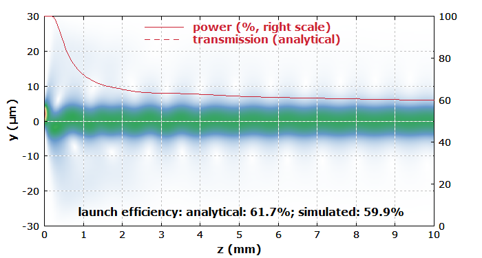
Figure 1 shows how the amplitude distribution evolves in the fiber. We see some wiggles, which result from a vertical offset of the incident beam position. Also, one can see how some of the light escapes from the core; this is the non-guided part which is lost after some length of fiber. The red curve shows how the power in the fiber drops. The final value is in good agreement with the analytical estimate.
We can also systematically vary the initial beam radius and see how the launch efficiency varies. This is shown by Figure 2. Here, the beam is assumed to be perfectly aligned to the core.
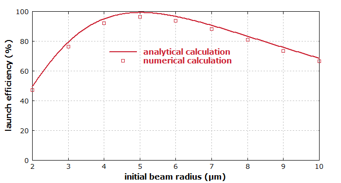
The numerical beam propagation results nicely agree with the analytical calculation. Note that they could also easily be carried out in more complicated cases. For example, one might have a fiber core which has no radial symmetry, any other kind of input beam profile, or a bent fiber.