Software > RP Fiber Power > Demos > HOM coupler

RP Fiber Power – Simulation and Design Software
for Fiber Optics, Amplifiers and Fiber Lasers

Example Case: Fiber Bragg Grating for Coupling into Higher-order Modes

Here we show how the numerical beam propagation feature of RP Fiber Power can be used for analyzing light propagation in fiber Bragg gratings, as long as no reflections are involved. This takes a little script programming, but you will see that it is actually quite straightforward.

Description of the Model

We first need to define the refractive index profile of the fiber from which the Bragg grating is made:

n_cl := 1.44  { cladding index }
n_co := n_cl + 2e-3  { core index }
r_co := 30 um  { core radius }
r_cl := 40 um  { region where n must be exactly constant }
L_f := 200 mm  { length of the simulated region }
 
n_f(r):= { index of pure fiber }
  if r <= r_cl then
    n_cl + exp(-ln(2) * (r / r_co)^8) * (n_co - n_cl)
  else
    n_cl

Instead of a simple step-index profile, we have used a supergaussian function.

Now we use this is an input for the mode solver in order to check how many modes we have:

calc set_n_profile("n_f", r_cl)
for m := 1 to m_max(lambda) do
 show "LP0" , m, ": ", beta_lm(0, m, lambda) * um:f6:" / µm"

We can then also use the mode solver for calculating the difference between the phase constants of the fundamental mode and of the targeted higher-order mode, from which we get the grating period required for effective coupling:

l_target := 0  { targeted mode }
m_target := 3
dbeta := beta_lm(0, 1, lambda) - beta_lm(l_target, m_target, lambda)
show "dbeta:  ", dbeta * um:f6:" / µm"
p := 2pi / dbeta
show "Period: ", p:d3:"m"

Now we define the three-dimensional refractive index profile of the fiber Bragg grating:

n_FBG(x, y, z):=  { index of fiber Bragg grating }
  begin
    var r;
    r := sqrt(x^2 + y^2);
    if r <= r_cl then
      n_cl + exp(-ln(2) * (r / r_co)^8) * (n_co - n_cl) * (1 + 0.1 * sin(dbeta * z))
    else n_cl;
  end

Now we set up the numerical beam propagation:

; Grid parameters for numerical beam propagation:
r_max := 4 * r_co
N_r := 2^7
dr := 2 * r_max / N_r
dz := 200 um
N_z := L_f / dz
N_s := 20  { number of sub-steps for each dz interval }
 
calc
  begin
    bp_set_device(1);
    bp_set_grid(r_max, N_r, r_max, N_r, L_f, N_z, N_s);
    bp_define_channel(lambda);
    bp_set_n_z('n_FBG(x, y, z)', 'z');
    bp_set_A0('A_lm_xy(0, 1, lambda, x, y)');  { fundamental mode as the input field }
  end

Finally, we can just use the function bp_I() for making a color plot of the resulting intensity distribution in the device. In addition, we can add some code for plotting the evolution of optical powers in the two modes:

diagram 1:
 
x: 0, L_f / mm
"z (mm)", @x
y: -r_max / um, +r_max / um
"y (µm)", @y
y2: 0, 100
"optical powers (%)", @y2
frame
hx
hy
 
! I_max := 1.5 * bp_I_max(0)
cp: color_I((bp_I(0, y * um, x * mm) / I_max)),
  order := yx
 
P_lm(l, m, z) := 
  { power in LP_lm mode at position z }
  abs2(int(int(bp_A%(x, y, z) * A_lm_xy(l, m, lambda, x, y),
    x := -r_max to +r_max step dr),
    y := -r_max to +r_max step dr))
 
f: 100 * P_lm(0, m_target, x * mm), yscale = 2,
  color = red, width = 1, ["LP", l_target, m_target, " power"]
 
f: 100 * P_lm(0, 1, x * mm), yscale = 2,
  color = blue, width = 1, "LP01 power"

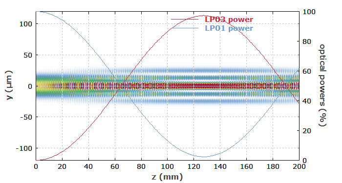
What we get is the following diagram:

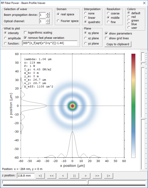
For interactively exploring the field profile, you can also use the interactive beam profile viewer:

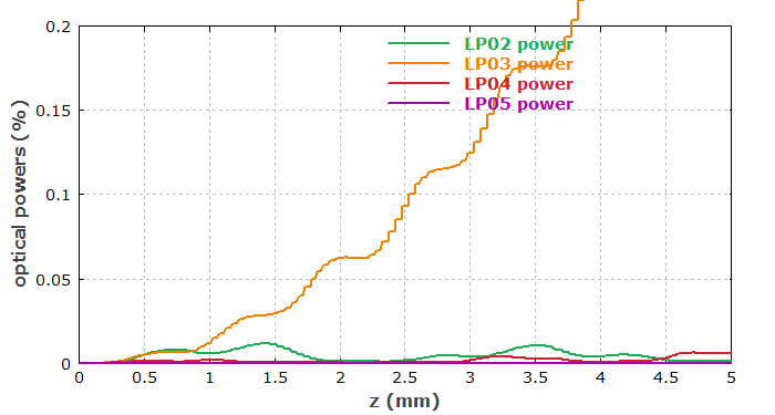
It is also interesting to check the evolution of mode powers in the very beginning of the fiber Bragg grating:

One can see that only the power in the LP₀₃ mode rises consistently, while the other mode powers oscillate up and down on very low levels. This is because the coupled contributions to the corresponding mode amplitude from different z positions in the device are normally out of phase – except for the one mode where we have compensated that phase change by using the right grating period.

Of course, it would be easy to change various details of the model or plot various other quantities. For example, you could study the effects of asymmetric grating structures, nearly degenerate modes in strongly multimode fibers, effects of bending, or whatever else may come to your mind!

(back to the list of example cases)