Software > RP Fiber Power > Demos > Fiber coupler

RP Fiber Power – Simulation and Design Software
for Fiber Optics, Amplifiers and Fiber Lasers

Example Case: Fiber Coupler

Here we show how RP Fiber Power can be used to analyze and optimize fiber couplers. We use the beam propagation feature to analyze a coupler with two inputs and two outputs, where two waveguides come close together over some distance such that their evanescent waves come into contact.

Description of the Model

We first need to define the refractive index profile of the device. We begin with defining a function for the y position of a waveguide as a function of the z coordinate:

y_c := 10 um  { vertical position of core in the coupling region }
y_i := 50 um  { vertical position of core in the input / output regions }
L_c := 2 mm  { length of the coupling region }
L_i := 10 mm  { length of the input and output region }
 
L_tot := 2 * L_i + L_c { total length }
y_co(z):= { vertical core position vs. z }
  if z <= L_i then
    y_c + (y_i - y_c) * 0.5 * (1 + cos(pi * z / L_i))
  else if z <= L_i + L_c then
    y_c
  else y_c + (y_i - y_c) * 0.5 * (1 + cos(pi * (L_tot - z) / L_i))

We then define the transverse profile of the refractive index of one waveguide as a super-Gaussian function:

n_cl := 1.45  { cladding index }
n_co := n_cl + 0.8e-3  { core index }
dn_co(r) := if abs(r) <= r_co then (n_co - n_cl) * exp(-(1.3 * r / r_co)^6)

From this we get the index profile of a single straight waveguide:

n_f(r) := n_cl + dn_co(r)

The whole coupler structure is defined as a three-dimensional refractive index distribution, and shown in Figure 1:

n_device(x, y,z) := 
  n_cl
   + dn_co(sqrt(x^2 + (y - y_co(z))^2))  { upper waveguide }
   + dn_co(sqrt(x^2 + (y + y_co(z))^2))  { lower waveguide }

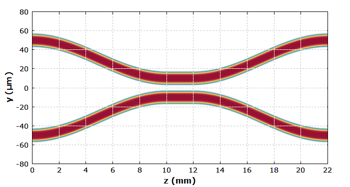
Of course, one could easily implement more sophisticated index profiles, taking into account the tapering of fibers in a fused coupler, or a twisted geometry.

We can now use the mode solver to calculate the modes of the single waveguides, and use these for the input to the upper waveguide, assuming that the input is in the LP₀₁ mode:

calc set_n_profile("n_f", r_co)
 
calc
  begin
    bp_set_device(1);
    bp_set_grid(x_max, N_x, y_max, N_y, z_max, N_z, N_s);
    bp_set_channel(lambda);
    bp_set_n_z('n_device(x, y,z)', 'trunc(y_co(z) / (0.2 um))');
    bp_set_A0('A_lm_xy(0, 1, lambda, x, y - y_i)');
  end

The index profile for the beam propagation is set with the function bp_set_n_z(). For each z value, the index distribution in the xy plane is recalculated only if the y position of the waveguides has changed by about 0.2 μm; this saves some computation time.

A few more lines of code, not shown here, define the numerical grid for the beam propagation. The grid has an extension of 50 μm in the x direction, 160 μm in the y direction, and 22 mm (the total length of the device) in the z direction. The numerical resolution in x, y and z direction is 1.56 μm, 1.25 μm and 10 μm, respectively.

Results

After these definitions, we can now simply use the function bp_I(x, y,z) for the optical intensity in the device. The square root of that (i.e., the amplitude distribution) is shown in Figure 2. One sees how light couples into the lower waveguide.

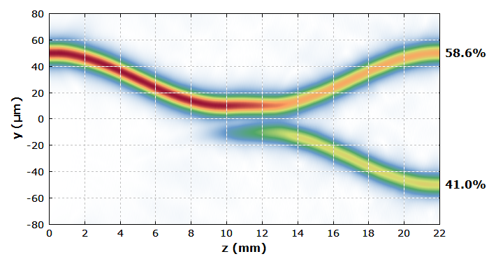
On the right side, we display the amount of power in the two outputs. We take only the LP₀₁ mode content, rejecting any stray light due to the bends, for example. This is achieved by calculating overlap integrals of the field distributions and the modes:

P_out_1() := { output power of port 1 }
  begin
    var cy, d, x1, x2, y1, y2;
    cy := dy * round(y_i / dy); { center position of the output port }
    d := 3 * r_co;
    x1 := -dx * round(d / dx);
    x2 := +dx * round(d / dx);
    y1 := cy - dy * round(d / dy);
    y2 := cy + dy * round(d / dy);
    abs2(int(int(bp_A%(x, y, z_max) * A_lm_xy(0, 1, lambda, x, y - y_i), 
      x := x1 to x2 step dx),
      y := y1 to y2 step dy));
  end

Due to the efficient implementation of the beam propagation in RP Fiber Power, a diagram as above can be generated within a few seconds on an ordinary PC.

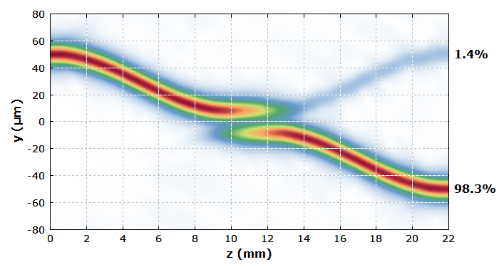
We can now reduce the distance between the waveguides in the coupling region from 20 μm to 16 μm. The light then mostly couples over to the lower waveguide:

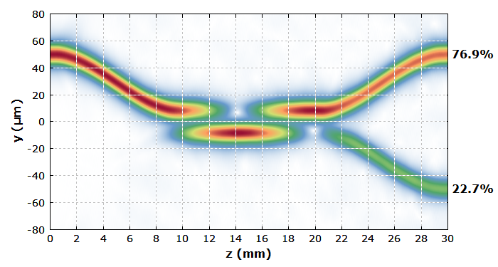
For the next diagram, we also increase the length of the coupling region from 2 mm to 10 mm. We then observe an oscillatory behavior in the coupling region:

For the previous coupler design, we now investigate the wavelength dependence. This is easily done with a few lines of script code (not shown here). The results are shown in Figure 5.

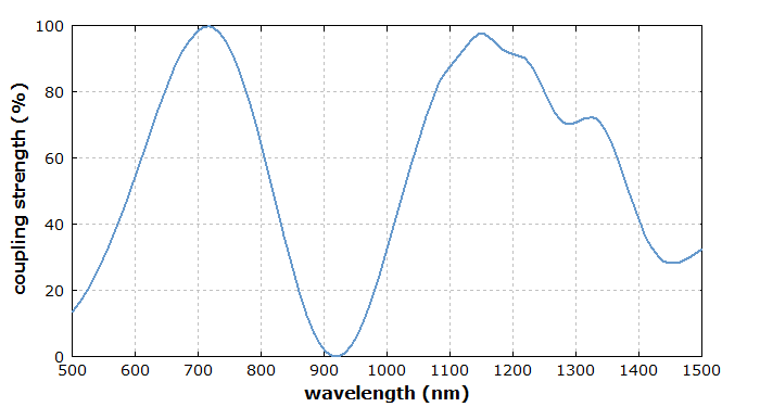
The somewhat strange shape of the curve in the longer-wavelength region results from bend losses of the waveguides, which get substantial in that region.

Making this diagram requires several minutes, because the full beam propagation has to be done for each wavelength.

We have actually neglected chromatic dispersion, i.e., the wavelength dependence of the refractive index; this could easily be included, e.g. based on Sellmeier formulas.

(back to the list of example cases)