Making Color Plots

Our software offers the simple command “cp:”. In many cases, it is sufficient to give it a mathematical expression which calculates the color value as a function of x and y. An example:

cp: color_I((sin(x) * cos(y))^2)

The predefined function color_I() converts values between 0 and 1 into color values, using a color scale which ranges from white (0) over blue (0.2), green (0.4), yellow (0.6), orange (0.8) to dark red (1).

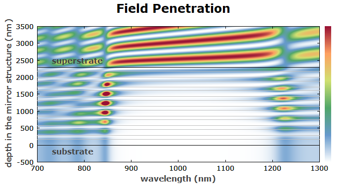
As another example, the following figure, taken from a case study on a Bragg mirror made with RP Coating, has used the same color scale:

The command used for making this color plot:

cp: color_I((R(x); E2(y)/4))  { color plot }

It again uses the predefined function color_I(), here in combination with the functions R(x) for the reflectivity of a mirror structure at a certain wavelength and the function E2() for the field intensity in the structure. What happens when the expression is evaluated for a certain value of x and y is the following:

• The reflectivity at the wavelength x (here in nanometers) is calculated. That also sets the field intensities throughout the structure. (The reflectivity value itself will be discarded.)
• Thereafter, the field intensity for the given depth y in the structure is returned.
• From that, the color value is calculated according by the color scale function.

That may seem to be a bit tricky in the beginning, but you quickly get used to that technique and can then make a wide range of nice color plots. You can also find a lot of them on this website.

Our software offers only two different predefined color scales through the functions color_I() and color_A(). You have seen the former, and the latter accepts a complex argument with a modulus up to 1; the complex phase determines the type of color, and the modulus determines the color saturation. That function can be useful for plotting complex amplitudes, as obtained e.g. from numerical beam propagation.

Of course, there are many other color scales which you might want to use. Here, you have full flexibility, because you can define your own arbitrary color scale functions. As an example, I show you how to implement the viridis color scale as explained here. That color scale is not defined through a simple formula, but rather through tabulated values, which you find in the file colormaps.py from https://github.com/BIDS/colormap/blob/master/colormaps.py.

Here is how you could define the new color function color_viridis(I) in our software:

; Define arrays for the RGB (red-green-blue) color values:
defarray R_viridis[0, 255]
defarray G_viridis[0, 255]
defarray B_viridis[0, 255]
 
; Read a table of data into those arrays:
j := -1
readlist R_viridis[j := j + 1], G_viridis[j], B_viridis[j]:
0.267004, 0.004874, 0.329415
0.268510, 0.009605, 0.335427
0.269944, 0.014625, 0.341379
; (253 more values not shown here)
 
; Define the color function, using the arrays:
color_viridis(I) :=
  begin
    global R_viridis[], G_viridis[], B_viridis[];
    var x;
    I := maxr(I, 0);
    I := minr(I, 1);
    x := I * 255;
    rgb(R_viridis~[x], G_viridis~[x], B_viridis~[x]);
  end

Once that is done, you can simply replace the function color_I() with color_viridis() in your scripts, and the new color scale is used!