Fiber Laser Model with More Than One Active Fiber

In principle, a software developer can try to add additional features to such forms. For our case, it might be useful to have some control where you can add additional active fibers to the laser resonator and perhaps switch between the parameters of these different fibers in order to edit all them. In addition, you would have to enter somehow how the different parts are connected. Well, that could in principle solve our example problem, but you can easily recognize the disadvantages of that approach:

• The more flexibility you try to achieve with such forms, the more complex and more difficult to use they will be. So you at risk to lose the most important advantage of forms: their ease of use.
• It is essentially impossible to offer anything a user might ever require – one reason being that the developer can hardly anticipate all that.

So there are severe limitations to the flexibility one can obtain that way. That is a problem with which some software developers are struggling severely.

A good solution to that fundamental problem is to use a script language, where the user can assemble any commands or functions to implement anything he or she needs.

To come back to our example case, we can use the following trick:

• Consider two separate devices: one with the left fiber, having an end reflector at the left end, and one with the right fiber, having an end reflector at the right end. Both receive some pump power, e.g. from the outer ends.
• Now consider some amount of signal (laser) power, entering the left fiber on its right end. That might still be amplified, reflected at the left end, and amplified again. Then it gets into the right fiber, will again be amplified, reflected, and amplified again. Now we are back to the original location, having done a complete resonator round trip.
• The problem is now only to determine the amount of signal power with which we should start. The correct level in the steady state is obviously the power for which the round-trip gain is zero. If we choose a too high value, the round-trip gain will be negative, since we have strong gain saturation. In the opposite case, the round-trip gain will be positive. Somewhere in between, there is the desired solution. So it is a simple one-dimensional root finding problem.

I just show you the part of the script code where the round-trip gain is calculated and where the root finding is done:

rt_gain(P_mid) := 
  { round-trip gain, starting from the middle of the resonator  }
  begin
    var P_rt, P_mid2;
    set_device(1);
    set_P_in(signal1_bw, P_mid);  { P_mid injected into the left fiber }
    P_mid2 := P_out(signal1_fw);  { that much comes back }
    set_device(2);
    set_P_in(signal2_fw, P_mid2);  { inject that into the right fiber }
    P_rt := P_out(signal2_bw);  { that much we get after one round trip }
    10 * lg(P_rt / P_mid);  { the round-trip gain in dB }
  end
 
P_mid := 
  if rt_gain(1 nW) > 0 then
    zero(rt_gain(P_mid),
         P_mid in [1e-9, P_pump1_fw_in + P_pump2_bw_in],
         xtol = 1e-9)

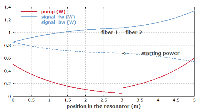
Also, I show you the generated diagram which shows the variation of optical powers within the laser:

It also shows the “starting power” which needs to be injected into the left fiber, coming from the place where the two fiber meet.

Of course, it would be easy to introduce further details like linear or nonlinear losses between the two fibers; the example shows that with the script language it becomes possible to implement a wide range of strategies to generate the results you need for your work.

For a beginner, it might be difficult to work out such tricks. However, good software comes with a helpful technical support. If you have our software and need something like that, I would personally come up with a suggestion for such a trick, and also implement it in an example script if required.