
![]()
RP Fiber Power – Simulation and Design Software
for Fiber Optics, Amplifiers and Fiber Lasers
| Overview | Features | Speed | Model |
| Data | Interface | Demos | Versions |
Example Case: Tapered Fiber
Here we investigate how light propagates in tapered fibers, i.e., fibers which have been heated and stretched such that the core dimension is reduced in some taper region.
Description of the Model
The reduction in fiber diameter is described with a simple function:
t_min := 0.5
t(z) := t_min + (1 - t_min) * 0.5 * (1 + cos(1 * 2pi * z / z_max))
When we later define the refractive index profile, we can easily use that function to modify a predefined two-dimensional function:
bp_set_n_z('n_f(sqrt(x^2 + y^2) / t(z))', 'z'); { index profile }
The numerical resolution needs to be chosen such that cladding modes are realistically modeled, because we must expect that some light is lost from the core in the tapered region.
Results
Initially, we assume a single-mode step-index fiber. The incident light is assumed to be fully in the guided mode (the LP01 mode) of the fiber. Figure 1 shows the amplitude distribution along the fiber. The gray curves illustrate the taper, reducing the fiber diameter in the middle by 50%. The red curve shows about 13% of the optical power are lost. This is because the LP01 becomes quite weakly guided in the taper region, and the taper is a bit too fast for an adiabatic transition.
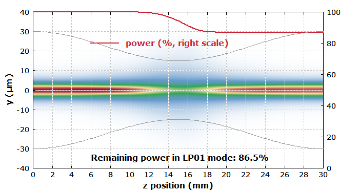
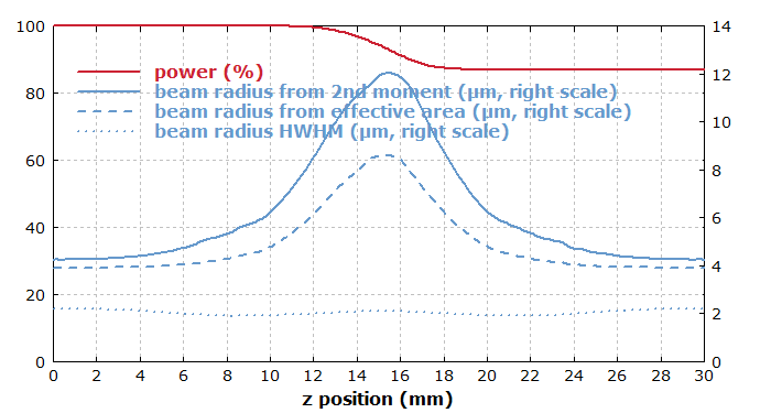
Figure 2 shows how various parameters evolve. Three different measures are used for the beam size:
- The beam radius calculated from the second moment of the intensity distribution. (The software offers a predefined function for that.) That value increases substantially in the taper region.
- The beam radius can also be calculated from the effective area, which is an entirely different definition. That value would be relevant for judging how strong nonlinear effects could be. It also increases in the taper region, but less strongly.
- The half width at half maximum (HWHM) of the intensity distribution. (Such a function can be user-defined easily with a few lines of script code.) That kind of beam radius even decreases a little in the taper region, at least initially, and overall shows only little variation. Note that it does not take into account the long “tails” of the intensity distributions of weakly guided modes.
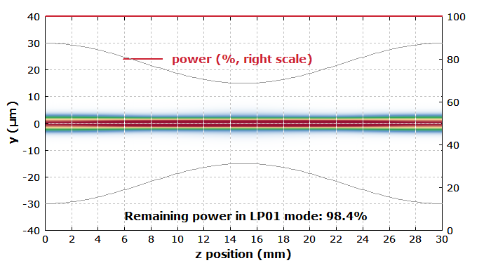
In a second simulation, we assume a fiber with doubled numerical aperture (0.2 instead of 0.1). That more strongly guiding fiber also supports LP11 modes – but not in the tapered region. If we launch the initial beam into the LP01 mode (as above), it can “survive” the tapered region without substantial losses, as it is guided quite strongly – see Figure 3. The beam size (not shown here) undergoes only quite moderate changes.
If we launch into the LP11 mode, the light is entirely lost in the taper region, as seen in Figure 4:
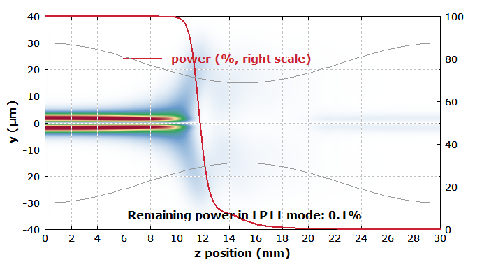
One sees in Figure 4 that reflections from the edges of the grid – a numerical artifact – are not completely suppressed. This, however, is no problem for the purpose of this investigation; only the detailed curve for the power drop and the calculated 0.1% transmission for the LP11 mode are not accurate – the latter should be essentially zero.